Introduction

This post is my learning exhaust from reading an exciting pre-print paper titled The Era of 1-bit LLMs: All Large Language Models are in 1.58 Bits about very efficient representations of high-performing LLMs. I am trying to come up to speed on deep learning after having been heads down in telecommunications systems and data at a startup since leaving research 13 years ago (!!!). This was a really fun way to take a deep dive, so I’m learning in public, so this post is the guide to the paper I wish I had before I read it :)

I dug into the details of this paper, and I'm hoping to help someone who is curious about the paper understand some of its nuances without digging through the references and reading up on all of the sub-topics.

In this post, I've offered some questions and criticisms of the paper, but please keep in mind that this is a pre-print about a great result, and so we should be reading it that way. There will, of course, be issues with a pre-print like this, and I'm overall very excited about the work the authors have done!

The punchline

At a very high level, the proposed architecture uses ternary weights during inference, which allows a dramatic increase in performance. Latency and memory consumption are (not surprisingly) dramatically better for the authors' models with ternary (-1, 0, 1) as opposed to full 16-bit FP weights. Here are plots from the paper:

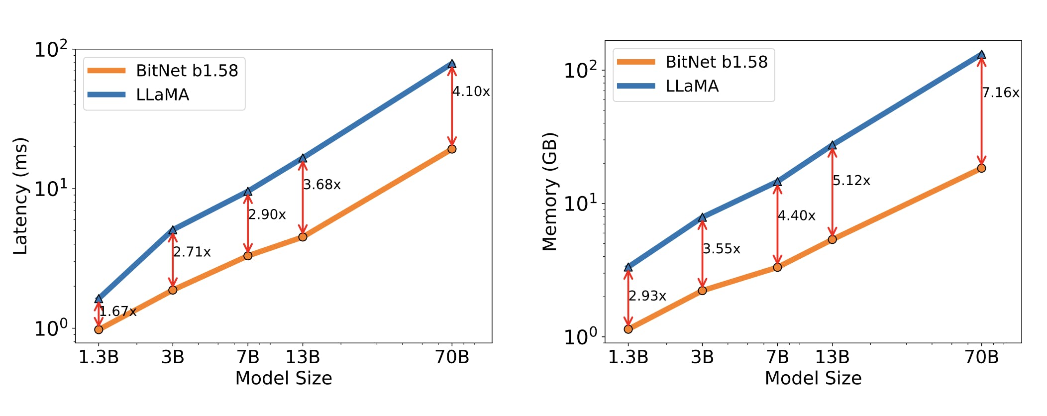
The punchline, however, is that the paper shows evidence that if we make a few tweaks to how we train ternary LLMs, they have the same performance as LLMs trained with 16-bit weights. The implication of this (if it is accurate) is that we can dramatically improve the performance of inference (but not training) without sacrificing quality.

This result is surprising (to me). Intuitively, by changing from a floating point representation to a ternary representation for the weights, we are dramatically reducing the amount of internal state that is available for the network to learn a mapping from input to output. On the other hand, researchers have spent a lot of effort investigating sparsity, with lots of results indicating that the active part of a neural network is often much smaller than the entire weight space (e.g. a lot of the weights are inactive, even in latent space). Maybe we pay for using fewer bits with denser networks? Or maybe higher precision in the weights is just unimportant because we add up a bunch of high precision activations, so we don't really need precise coefficients to blend the features from the previous layers?

Before we discuss the why, though, let's talk about the what and the how.

The key algorithmic contributions

The concept of a binary weight neural network is not new at all. I’m not an expert, so I won’t point you to a particular survey, but papers abound. Ternary weights have also been studied a lot because they allow (as the authors note in their introduction) the weights to mask features from previous layers by using the 0 values for some weights.

Regardless, the authors made some important decisions in the design that seem to have contributed to the model's effectiveness. Lets take a close look at how it works, particularly how it differs from regular, floating-point-weight models.

Most of the details about the model itself actually come from their previous paper, called BitNet: Scaling 1-bit Transformers for Large Language Models. The authors follow the same architecture in both papers, with the primary difference being using ternary vs. binary weights.

Here is a block diagram from the BitNet paper that explains the modified Transformer architecture at a high level.

In other words they have replaced the standard linear blocks with the BitLinear block from the paper. Let's take a look at the way that BitLinear works in the context of the forward and backward passes.

The forward pass

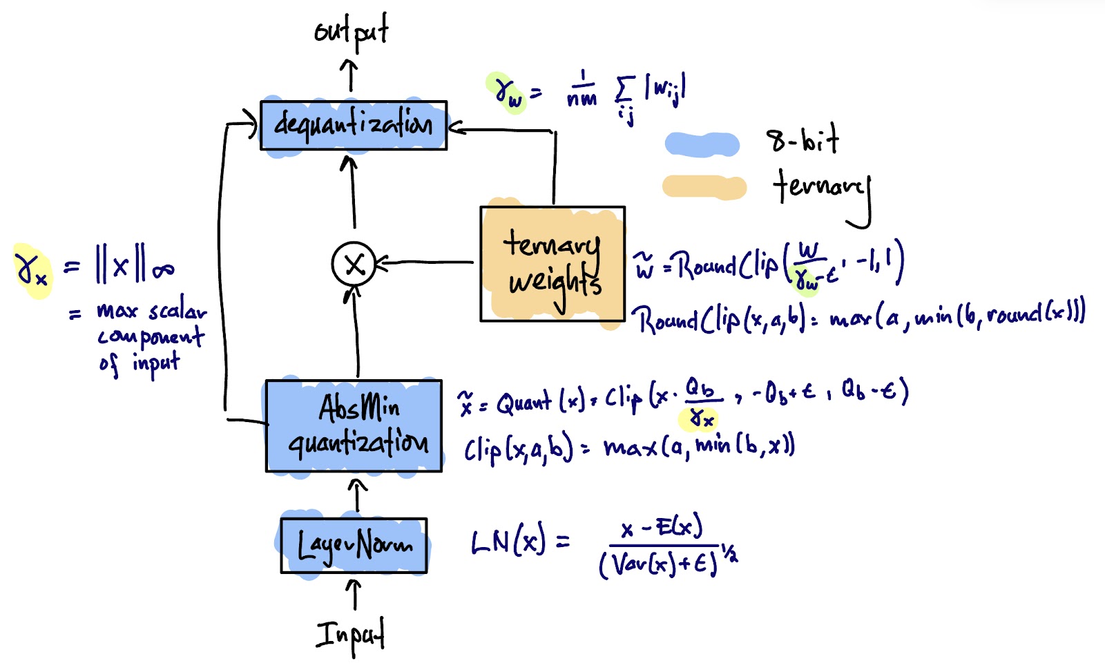
I reproduced this diagram from the BitNet paper. It shows the BitLinear block (see the previous diagram for context). I added the various formulas from the BitNet paper and some of the references from that paper. I also unified the notational differences between the various papers.

The first important architectural decision the authors made is to only use ternary (or binary) weights; e.g. don't use binary/ternary activations. The consequence of this decision is that information propagates through the network at higher fidelity (actually at 8-bit precision), and only the MLP transform layers (including attention layers) are ternary.

In other words, we can add, subtract or ignore features from the previous layers, but not change their "strength". For example, the \(i\)th activation at layer \(L\) might look like this

$$a^{(L)}_i= a^{(L-1)}_1-a^{(L-1)}_2 +a^{(L-1)}_4 + \cdots$$

instead of something like

$$a^{(L)}i= w^{(L)}{1,i} a^{(L-1)}{1} + w^{(L)}{2,i} a^{(L-1)}_{2} + \cdots$$

where \(w_{j,i}\) is the weight between \(a_j^{(L-1)}\)and \(a_i^{(L)}\).

Here is a diagram of attention weights from an article that describes the bertviz tool. You can play with great interactive visualizations in the notebook they link. (Note: these are not the weights from the BitNet models. I would love to follow up with a visualization like this of the weights from the actual models)

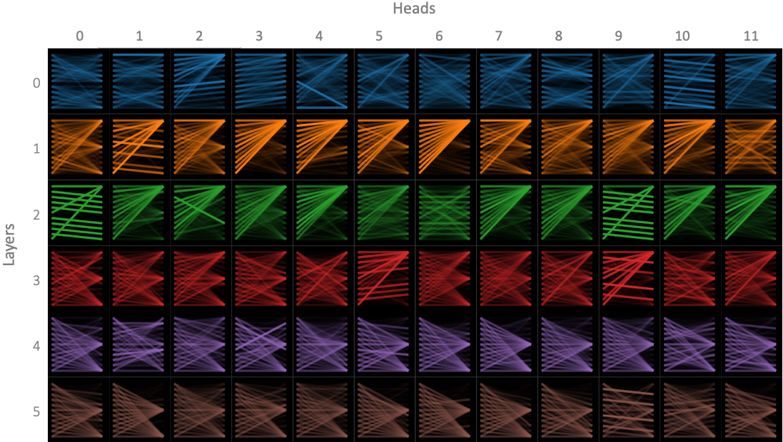
Notice that many of the plots are somewhat sparse, and that the intensities tend to be either on or off. This is probably partly due the way the weights are visualized, but what stands out for me is that some are on, some are off, with not a lot in between for many weights. Perhaps this visual intuition goes some way to explaining why ternary weights are good enough? Maybe we just need to activate or not activate upstream features, and not be too concerned with how much we activate them (although the sign of the activation seems to matter too)?

A recent paper called Physics of Language Models: Part 3.3, Knowledge Capacity Scaling Laws provides some more evidence about this. The paper shows that common Transformer architectures have a total information capacity of about 2 bits per parameter. They also show that this holds even in modified models that don't have any MLP (linear) layers, which suggest that information can move into other parts of the model during training. This raises the question of whether a ternary-weight model will reach its information capacity sooner than 2 or more bit model, since 1.58 < 2 (to state the obvious). Thanks to @picocreator for pointing me to this paper!

Other details

The LayerNorm layer is designed to preserve variance from the input in the output. The BitNet paper refers to Layer Normalization, which explores how this normalization improves model performance during training.

The quantization itself works basically as you would expect, and the formulas are in the diagram above, again from the BitNet paper. The one important thing to note is that during quantization, the weights and activations get scaled to the total range of the quantization (\(\gamma_w\) and \(\gamma_x\) respectively). We use these values to re-scale the outputs to the same scale as the inputs. This reportedly improves stability during training.

Additionally, because the quantization requires calculating\(\gamma_x\) and LayerNorm requires calculating the \(\mathbb{E}[x]\) and \(\sigma_x\), the naive implementation would require extra inter-GPU communication in order to split the model across GPUs using model parallelism. The BitNet paper introduced "group quantization," which basically just uses the approximate \(\gamma_x\), \(\mathbb{E}[x]\) and \(\sigma_x\) values calculated over the activations local to the GPU. They found that it has minimal impact on performance.

The backwards pass

One of the most interesting things about the BitNet b1.58 models is that they actually use full FP16 precision weights during the backwards pass in order to ensure that we have a reasonable gradient for our optimizer. If we used ternary weights in our optimizer, most optimization steps would not have any gradient for most weights, which would make it difficult figure out how to change our weights in order to improve our loss.

The consequence of this decision is that we are keeping both a full precision and ternary copy of weights during training. This makes training less memory efficient than in a standard Transformer. Since large models are bottlenecked on memory bandwidth, this has a significant impact on training performance.

I would have liked to see the authors explore this tradeoff more. We'll get to that in the Scaling Laws section below.

The authors also claim in their supplemental notes, that "1.58 bit models can save a substantial amount memory and communication bandwidth for distributed training," but don't elaborate much on why. I don't understand their argument here, since they presumably would need to transfer the full precision weights to other nodes.

Finally, the authors mention briefly that they use a "straight-through" estimator of the weight gradients, which means that they just ignore the quantization when calculating the gradient. This is because the quantization makes the function non-differentiable. Previous research they cite has found that the straight-through estimator does about as well as more complex methods, and is trivial to implement.

Post training quantization

In the original BitNet paper, the authors compared 1-bit quantization using BitNet to to various methods of post-training quantization. The key difference between BitNet / BitNet b1.58 and post-training quantization is that the forward pass is done using the quantized binary / ternary weights, so that the weights and activations are trained to be accurate in the quantized state-space.

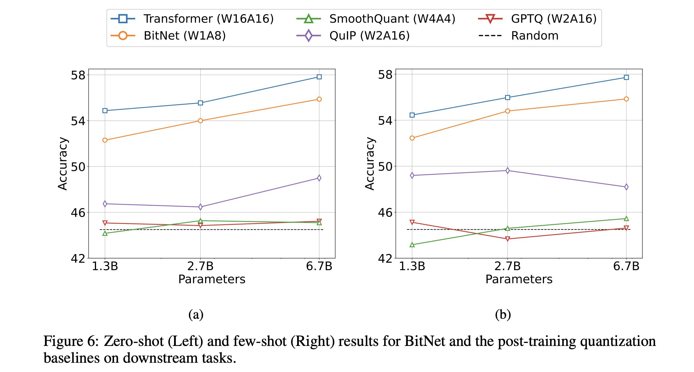
The blue line shows the accuracy of a FP16 transformer trained using the same training regime as the 1-bit BitNet across various sizes. Three post-training quantizations on the FP16 transformer are also shown. The authors do not explain exactly how they measure accuracy, but presumably it is the average of the benchmarks they ran on these models.

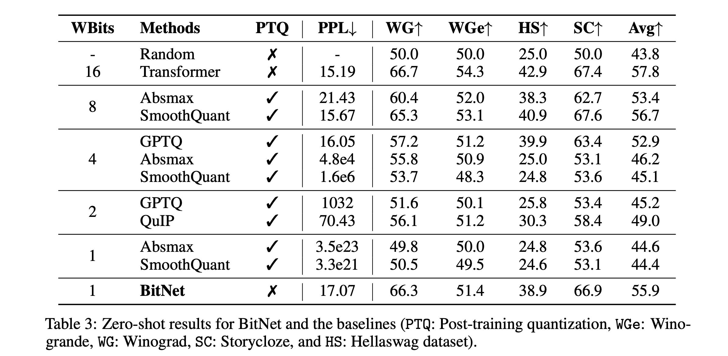
This table shows perplexity and accuracy on other data sets:

• Winograd - a benchmark of questions that measure the ability to reason about complex statements

• Winogrande - a larger and more difficult version of Winograd

• Storycloze - choose the correct ending of a four sentence story

• Hellaswag - choose the correct ending of a story, curated by adversarial filtering to identify examples that are hard for NLP algorithms

Similar to the accuracies in the plot above, BitNet slightly more poorly that the FP16 transformer, whereas the post-quantization methods degrade significantly as we remove bits. Note that at 1 bit, Absmax and SmoothQuant both perform about the same as random chance.

I think the authors really should have repeated this comparison more explicitly for the BitNet b1.58 paper. The sizes of models in the papers are not comparable except for the 3B model, so it's hard to compare the results.

Model inference quality

As noted in the introduction, the model performance is the surprising part of this paper. The authors trained a full FP16 LLaMa-architecture LLM (e.g. the same architecture without the quantized weights and activations) to compete with their BitNet b1.58 version at three sizes: 700M, 1.3B, and 3B parameters. They train for 100B tokens using the RedPajamas data set. They also trained a BitNet b1.58 model at 3.9B parameters. Presumably they chose this size in order to illustrate that a small delta in parameter count allows them to beat the 3B model on all of the benchmarks they ran while requiring significantly less memory and inference latency.

This table comes from the BitNet b1.58 paper. The perplexity for the BitNet b1.58 3B and 3.9B models is slightly lower than for the 3B LLaMA model. This is certainly interesting and surprising because it is not the case for smaller models. Since perplexity is a measure of the confidence of the model, if it were smaller for all of the BitNet b1.58 models then we might guess that it is simply overconfident due to some artifact of the quantization and/or training process.

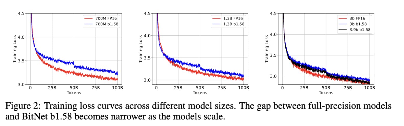
These plots come from the supplemental notes. The drop in loss at 50B tokens is due to a change in the learning rate and weight decay schedules at that time. As the caption notes, the gap between the training loss for the models gets lower as the size of the models get larger. This suggests that the lower perplexity is not due to overconfidence. On the other hand, the authors did not show the validation loss, so perhaps the lower loss is due to overfitting?

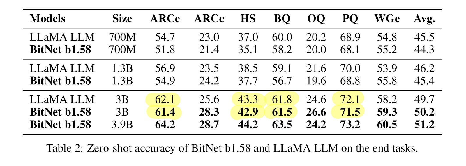
This table, from the BitNet b1.58 paper, shows model performance across a range of inference quality benchmarks. The average performance of the 3B model is higher than the FP16 model, although this is probably in the noise. In fact, the reproduced results (shown below) show the average results being very slightly worse for the 3B model. I don't think this impacts the result: the inference quality of the model is very close to the full precision model, especially considering that LLM benchmarks are notorious for not reflecting real inference quality anyways.

Other details

As we would expect, the memory usage and latency are better with the BitNet b1.58 models. Note that the paper says "The 2-bit kernel from Ladder is also integrated for BitNet b1.58," which references a poster at a conference. I was unable to find any other information on Ladder, so we have to presume that they are using a kernel that can represent ternary integers as 2-bits and efficiently load and operate on them. I hope the authors publish the Ladder 2-bit kernel in their final publication.

Reproduced results

These results sort of seem too good to be true. How can we get the same performance as full precision model with such low precision weights? Maybe the researches just made a mistake like leaking validation data?

Fortunately, someone (Nous Research?) was able to replicate the core results and published the models and a summary of their findings.

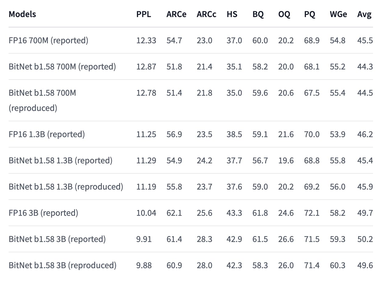
The replicated results are very close to the reported results in almost every case, which is very promising. This rules out a basic mistakes such as data leaks. It does not necessarily rule out methodological or fundamental epistemological errors, but the people who replicated the results were presumably thinking about these as well, and presumably would have reported flaws they discovered.

2T token model

The authors also trained a 2T token model in order to validate scalability, by which I think they mean to validate that a model with ternary weights does not stop improving earlier than a FP16-weight model. They followed the same data recipe as StableLM-3B-4E1T, which basically repeated a 1T token data set 4x. They seem to have use the data from the continuous validation dynamics section of the technical report to compare the halfway-point in the StableLM-3B-4E1T training (e.g. at 2T tokens) to their own results.

While this seems like a reasonable comparison, this is not at all clear in the text of the paper, and should be made explicit. It does raise some minor concerns, since the mid-training results lack a cooldown period, and the "validation dynamics across our hold-out set" of the StableLM-3B-4E1T training run are unclear. There may be other problems with this methodology that someone more experienced would notice as well.

In any event the above table shows that BitNet b1.58 3B performs comparably to StableLM-3B after 2T tokens of training. I don't think we can presume that BitNet b1.58 3B would actually perform better than StableLM-3B after 2T tokens of training if the Stability AI team had planned to stop training after 2T tokens, but the result does seem to suggest that BitNet b1.58 3B does indeed continue to improve in a similar way to a FP16-weight model.

Again, the authors should be more explicit about their methodology, since it raises uncertainty about the validity of their results.

Inference performance

The validation of on-par performance of the ternary weight models goes hand in hand with the dramatic improvement in inference latency and memory consumption. These two results together, if correct, represent a significant advance in the cost/accuracy Pareto front. Particularly interesting is the observation that the improvement over a FP16 model increase as the size of the model increases, (see the plot of inference latency and memory consumption vs model size above) since the Linear layers increasingly dominate the inference cost.

The paper also discusses energy consumption since this is a better metric of computational cost than FLOPs for this study, considering that the BitNet b1.58 models get some of their advantage by eliminating the need for most of the FLOPs in the weight multiplications.

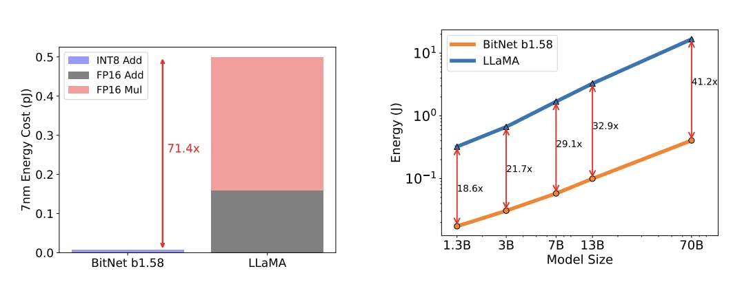
While these numbers are impressive, they mostly just reiterate, in combination with the latency numbers above, that the bottleneck for inference is not compute.

New hardware?

The abstract and conclusion mention new hardware. As we discussed above, it seems likely that the most significant improvements would come from improvements in memory utilization by using special circuitry to pack, unpack and operate on ternary weights. Since an efficient encoding would enable 10 weights per 16 bits, whereas a 2-bit representation would only allow 8 weights per 16 bits, the improvement would be limited to 25%.

In as much as memory rather than compute is the bottleneck for LLM inference, this does not seems worth the enormous expense of specialized ternary circuitry, especially considering that it would limit the chip's usefulness for non-LLM applications.

Scaling laws

Following from the discussion in the inference performance section above, the improvement in inference cost will be driven by memory utilization, or perhaps total latency. Since previous scaling law papers have used FLOPs as an approximate proxy for cost, we can do a back-of-the-envelope approximation of the impact of BitNet b1.58 on cost by just using the latency or memory deltas to adjust the number of inference "FLOPs" in the scaling law.

For the unfamiliar, the Chinchilla paper found that cost optimal training regime, without consideration for inference costs, is about 20 training tokens per model parameter.

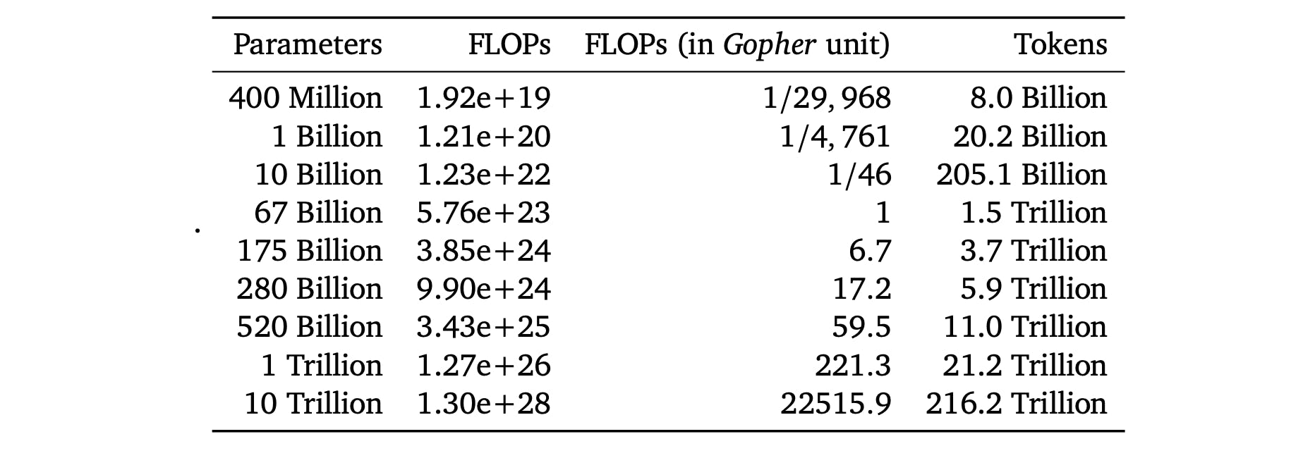
The above table, reproduced from the Chinchilla paper, shows the number of training tokens for various model sizes needed to optimize training costs.

Since the release of the Chinchilla paper, attention has shifted towards inference cost as companies have put models into production.

The above equation, from Beyond Chinchilla-Optimal: Accounting for Inference in Language Model Scaling Laws uses the common rule of thumb that Transformer-architecture LLMS need \(6N\)FLOPs per training token, and \(2N\)FLOPS per inference token. In this equation, the \(N\)values represent the number of model parameters, and the \(D\) values represent the number of tokens.

Note that if we don't do any inference with our model, then this equation reduces to the Chinchilla-optimal cost. So, intuitively, we are just scaling the second term as our inference becomes more efficient, and getting closer to the Chinchilla-optimal token/parameter ratio.

So for our back-of-the-envelope calculation, we can adjust the 2nd term in the equation above by our memory or latency factor from the very first plot in this post, reproduced above for clarity.

There's a lot to keep in our heads here, so as an example, assuming a 70B model, then we would divide the inference tokens term in the equation above by 4.1 if we are assuming cost scales with latency, or 7.16 if we assume that cost scales with memory utilization

The above plot, also from inference scaling law paper show the adjustment factor to apply to the Chinchilla-optimal model configuration for given target training loss, and given number of inference tokens.

Again, this is a lot to keep in our heads, so let's continue with our example. Since training loss is highly dependent on all sorts of factors, we'll treat it as "funny money" and just pick something that seems reasonable, like 2. This seems reasonable based on the loss curves from the StableLM-3B-4E1T Technical Report.

Now, lets take a look at the contour plot (the ratio of cost-optimal pre-training tokens to Chinchilla optimal tokens). If we look at the 2.0 training loss line, we can look up some total number of inference tokens that we expect to pay for. Let's call it 10e13 = 10T. Now if we adjust the number of inference tokens by the latency reduction factor of 4.10, then we need to look \(log_{10}(4.10)\approx0.6\) ticks on the graph to the left of the 10e13 line (green arrow). This puts us right around the 2x contour. So this tells us that we should use about 2x the chinchilla optimal number of parameters, which is about 1400B x 2 = 2800B training tokens.

We can do a similar exercise if we have a given number of training tokens and need to know how to pick a cost optimal size model at a given loss (see the paper for details).

This is pretty awesome! In essence, we need fewer training tokens to get to cost optimal for a known number of inference tokens. Of course, the number of inference tokens is hard to project for a proprietary model, let alone an open source model. This scaling law will also run out steam in the limits of model sizes and token counts, but it's not clear from the paper where those limits are. But it is certainly useful to develop an intuition for the impact of the BitNet b1.58 models on scaling.

Tying it up

Someone trained a set of models using the recipe from the authors. These models have the full FP16 weights, which is great because we can use them to study the relationship between the full precision weights and the quantized ones. It does mean, however, that if we want to get the performance benefits of the quantization, we have to actually quantize the FP16 weights down to ternary and update the inference code to take advantage of it.

Fortunately, HuggingFace user kousw has quantized the 3B model and written the code to do inference on it! I have a demo notebook here: https://colab.research.google.com/drive/1KDQBle0hByR9oB1b9MVx9nmaDiHTr8_9

In any event, this paper does a great job of telling us about an exciting result, but leaves a lot to the reader to dig up for themselves. This is fine for a pre-print, I just hope they will flesh out the paper a bit more before publishing it. I would have liked to see

• a more direct comparison of the quantization results

• more explicit exposition of the scaling law claims

• a better explanation of their arguments about hardware

Perhaps more importantly, we got a lot of what, a bit of how, and very little why.

• why does post quantization work better? They have a hypothesis in their supplemental notes ("This is because PTQ can only quantize model weights around the full-precision values, which may not necessarily be where the global minima of the low-precision landscape lie.") The authors should design an experiment to support their hypothesis, or cite research on it more clearly.

• Why does ternary work just as well as FP16? Why not binary?

  • Since higher precision activations seem to be important, does information move from the weights into other places like biases or other parameters? We could test this by measuring the entropy in the weights, biases and activations in an unquantized vs. quantized weight training regime

  • For ternary vs. binary, can we correlate errors to the inability to mask features?

• Why does ternary work better than FP16?

  • Is this a kind of regularization?

• Does using a ternary weighted model have a lower information capacity than models with more bits per weight? The authors state in the supplemental notes regarding use all 4 values of the 2-bit representation "While this is a reasonable approach due to the availability of shift operations for -2 and 2 to eliminate multiplication, ternary quantization already achieves comparable performance to full-precision models. Following Occam’s Razor principle, we refrained from introducing more values beyond {-1, 0, 1}." Perhaps, given the results from Physics of Language Models: Part 3.3, Knowledge Capacity Scaling Laws, this decision is premature?

They have hypotheses, but don't explore them, and so this reads as a (very interesting) technical report, and not a research paper. That's fine for a pre-print, but I would love to know more about why, and not just what.

In conclusion, what a great result! I look forward to hearing more from the authors, hopefully some followup on the things I mentioned above, and of course, their models and code!

Resources

• The Era of 1-bit LLMs: All Large Language Models are in 1.58 Bits - the paper itself

  • Supplemental notes - details about how to replicate their results, and answering some of the questions they got as a result of the pre-print

  • BitNet: Scaling 1-bit Transformers for Large Language Models - the preceding paper. You probably need to read this paper as well if you want to understand this one

  • Layer Normalization - the source of their LayerNorm stage

  • The paper page on HuggingFace with some great discussion about the results and models

• The replicated models on HuggingFace, including some replicated evals

  • The quantized 3B model for faster inference

  • My notebook to fiddle around with the quantized model

  • StableLM-3B-4E1T Technical Report - the presumptive source of the 2T token comparison that they make to argue that they continue to scale as the number of training tokens increasses

• Scaling laws

  • Chinchilla paper

  • Beyond Chinchilla-Optimal: Accounting for Inference in Language Model Scaling Laws

  • Physics of Language Models: Part 3.3, Knowledge Capacity Scaling Laws - a recent analysis of the knowledge capacity of transformer-based models

• Meta stuff

  • learning in public - a great post by @swyx about how and why to share your learning journey with others

  • learning exhaust - a great post by @swyx about how to improve your learning by taking advantage of the artifacts you produce while learning